Surface Water Level Monitoring with Sentinel-2

Table of contents¶

Introduction
Setup
Access data
Visualize datacube sample
Cloud masking
NDWI
Water detection
Water surface area extraction

Introduction¶

This notebook demonstrates how to estimate and visualize surface water area measurements at Santa Giustina lake, Italy, using Sentinel-2 data stored in EOPF-Zarr format.

The lake¶

Lago di Santa Giustina is an artificial lake located in the Trentino region of northern Italy. It was created in the 1950s by damming the Noce River for hydroelectric power generation. The lake is situated at an elevation of approximately 500 meters above sea level and has a surface area of about 3.5 square kilometers.

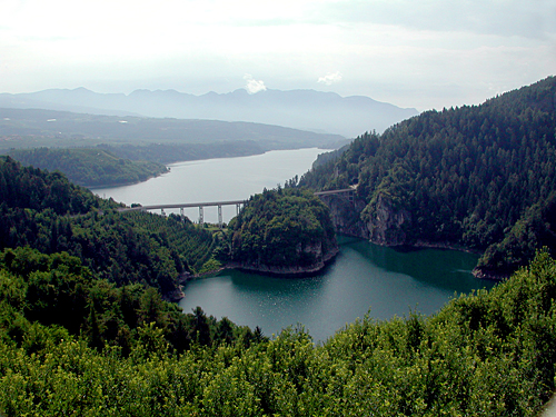
Image source: By Mosco - Own work, CC BY-SA 3.0, https://commons.wikimedia.org/w/index.php?curid=5144281

Setup¶

Start importing the necessary libraries

import xarray as xr
import geopandas as gpd
import matplotlib.pyplot as plt
import numpy as np

import pystac_client

from rasterio.features import geometry_mask

from skimage.filters import threshold_otsu
import pandas as pd
from skimage import measure

from pyproj import Transformer

import dask
from dask_gateway import Gateway

import warnings

warnings.filterwarnings("ignore", category=UserWarning)
warnings.filterwarnings("ignore", category=DeprecationWarning)

"""
gate = Gateway("https://dask.user.eopf.eodc.eu",
               proxy_address="tls://dask.user.eopf.eodc.eu:10000",
               auth="jupyterhub")
"""

# Dask Gateway automatically loads the correct configuration.
# So the code below is identical to the comment above
gate = Gateway()
cluster = gate.new_cluster()
cluster.scale(8)

client = cluster.get_client()
client

Access data¶

Query the EOPF Sentinel-2 STAC Collection for the area and time of interest.

catalog = pystac_client.Client.open("https://stac.core.eopf.eodc.eu")
bbox = [
    11.003288060439315,
    46.34055268553584,
    11.10369555555596,
    46.40183319621778,
]
items = list(
    catalog.search(
        collections=["sentinel-2-l2a"],
        bbox=bbox,
        datetime=["2020-12-31", "2024-01-01"],
    ).items()
)
print(f"items found: {len(items)}")

items found: 434

Combine the products into a single datacube:

%%time


def reproject_bbox(bbox, src_crs="EPSG:4326", dst_crs="EPSG:32632"):
    transformer = Transformer.from_crs(src_crs, dst_crs, always_xy=True)
    xmin, ymin = transformer.transform(bbox[0], bbox[1])
    xmax, ymax = transformer.transform(bbox[2], bbox[3])
    return [xmin, ymin, xmax, ymax]


def load_tile(item, bbox_ll):
    href = item.assets["product"].href
    ds = xr.open_datatree(href, engine="zarr", chunks={}, mask_and_scale=True)

    dst_crs = item.properties.get("proj:code")
    if dst_crs is None:
        raise ValueError(f"No proj:code in item {item.id}")

    utm_bbox = reproject_bbox(bbox_ll, dst_crs=dst_crs)

    ds_ref = (
        ds["measurements"]["reflectance"]["r20m"]
        .to_dataset()[["b02", "b03", "b04", "b8a"]]
        .sel(x=slice(utm_bbox[0], utm_bbox[2]), y=slice(utm_bbox[3], utm_bbox[1]))
        .expand_dims(time=[item.datetime])
    )

    ds_scl = (
        ds["conditions"]["mask"]["l2a_classification"]["r20m"]
        .to_dataset()
        .sel(x=slice(utm_bbox[0], utm_bbox[2]), y=slice(utm_bbox[3], utm_bbox[1]))
        .expand_dims(time=[item.datetime])
    )

    return xr.merge([ds_ref, ds_scl])


delayed_results = [dask.delayed(load_tile)(item, bbox) for item in items]
results = dask.compute(*delayed_results)

# Get CRS from STAC item
crs = items[0].properties.get("proj:code")

datacube = xr.concat(results, dim="time").sortby("time")

datacube = datacube.rio.write_crs(crs, inplace=True)
datacube

Open the geoJSON file containing the lake boundaries:

lake_gdf = gpd.read_file("./geojson/lago_santa_giustina.geojson")
lake_gdf = lake_gdf.to_crs(crs)

Visualize datacube sample¶

In this section we visualize an RGB composite for a random date and use the lake polygon as an outline to see if it is aligned correctly.

datacube_sample = datacube.isel(time=50)

rgb = datacube_sample[["b04", "b03", "b02"]].to_dataarray(dim="band")

rgb = rgb.assign_coords(band=["red", "green", "blue"])

vmin, vmax = 0, 0.25
rgb_scaled = (rgb - vmin) / (vmax - vmin)
rgb_scaled = rgb_scaled.clip(0, 1)

rgb_img = rgb_scaled.transpose("y", "x", "band").values

fig, ax = plt.subplots(figsize=(8, 8))
ax.imshow(
    rgb_img,
    extent=[
        float(rgb.x.min()),
        float(rgb.x.max()),
        float(rgb.y.min()),
        float(rgb.y.max()),
    ],
)

lake_gdf.boundary.plot(ax=ax, edgecolor="yellow", linewidth=2)
ax.set_title("RGB composite with lake boundary overlay")
ax.axis("off")
plt.show()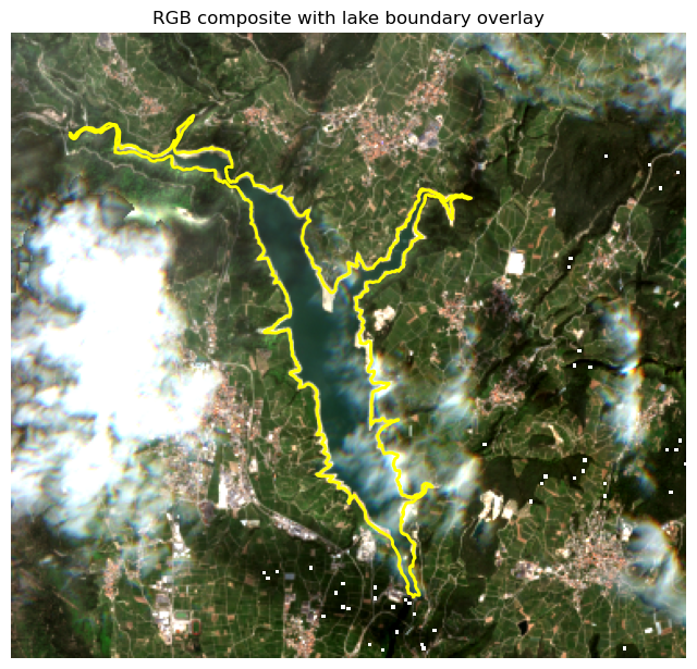

Cloud masking¶

In this section we apply the scl band to mask out the clouds. We visualize the same RGB composite as before, but with the mask applied.

valid_classes = [2, 4, 5, 6]

mask = datacube["scl"].isin(valid_classes)

datacube_masked = datacube.where(mask)

datacube_sample = datacube_masked.isel(time=50)

rgb = datacube_sample[["b04", "b03", "b02"]].to_dataarray(dim="band")

rgb = rgb.assign_coords(band=["red", "green", "blue"])

vmin, vmax = 0, 0.25
rgb_scaled = (rgb - vmin) / (vmax - vmin)
rgb_scaled = rgb_scaled.clip(0, 1)  # keep in [0, 1]
rgb_img = rgb_scaled.transpose("y", "x", "band").values

fig, ax = plt.subplots(figsize=(8, 8))
ax.imshow(
    rgb_img,
    extent=[
        float(rgb.x.min()),
        float(rgb.x.max()),
        float(rgb.y.min()),
        float(rgb.y.max()),
    ],
)
lake_gdf.boundary.plot(ax=ax, edgecolor="yellow", linewidth=2)
ax.set_title("Cloud-masked RGB composite")
ax.axis("off")
plt.show()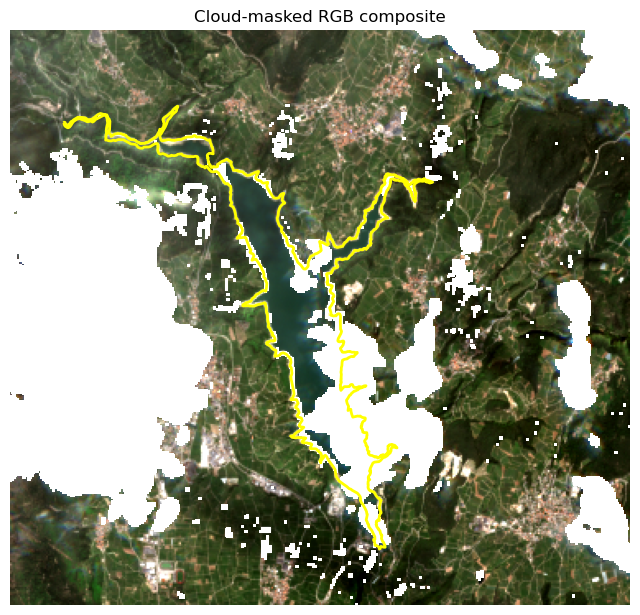

We keep only the dates with a cloud coverage less than 5% over the lake:

valid_classes = [4, 5, 6]
threshold = 0.05

datacube_lake = datacube.rio.clip(lake_gdf.geometry, lake_gdf.crs)

clear_mask = datacube_lake["scl"].isin(valid_classes)

clear_fraction = clear_mask.mean(dim=("y", "x")).compute()

mask_good = clear_fraction >= threshold

datacube_clear = datacube_lake.isel(time=mask_good)
datacube_clear

NDWI¶

Water detection is performed using the Normalized Difference Water Index (NDWI), which utilizes the green and near-infrared (NIR) bands of the Sentinel-2 imagery. The NDWI is calculated as follows:

NDWI = \frac {GREEN - NIR} {GREEN + NIR}

(1)

ndwi = (datacube_clear["b03"] - datacube_clear["b8a"]) / (
    datacube_clear["b03"] + datacube_clear["b8a"]
)

Water detection¶

The water area is selected applying Otsu Thresholding:

def otsu_mask(arr):
    arr = np.clip(np.nan_to_num(arr, nan=0.0), -1, 1)

    valid = arr > -0.2
    if np.count_nonzero(valid) < 10:
        return np.zeros_like(arr, dtype=bool)
    try:
        thr = threshold_otsu(arr[valid])
    except Exception:
        thr = 0.0
    thr -= 0.05

    return arr > thr


ndwi = ndwi.chunk({"x": -1, "y": -1})
water_masks = xr.apply_ufunc(
    otsu_mask,
    ndwi,
    input_core_dims=[["y", "x"]],
    output_core_dims=[["y", "x"]],
    vectorize=True,
    dask="parallelized",
    output_dtypes=[bool],
)

water_masks.compute()

water_masks

Sample visualization of computed water mask:

target_time = "2021-04"

datacube_full_rgb = datacube.sel(time=target_time, method="nearest")[
    ["b04", "b03", "b02"]
].to_dataarray("band")
datacube_full_rgb = datacube_full_rgb.assign_coords(band=["red", "green", "blue"])

vmin, vmax = 0, 0.25
rgb_scaled_full = (datacube_full_rgb - vmin) / (vmax - vmin)
rgb_scaled_full = rgb_scaled_full.clip(0, 1)
rgb_img_full = rgb_scaled_full.transpose("y", "x", "band").values

water_mask_da = water_masks.sel(time=target_time, method="nearest")

fig, ax = plt.subplots(figsize=(8, 8))
ax.imshow(
    rgb_img_full,
    extent=[
        float(datacube_full_rgb.x.min()),
        float(datacube_full_rgb.x.max()),
        float(datacube_full_rgb.y.min()),
        float(datacube_full_rgb.y.max()),
    ],
)

water_mask = water_mask_da.values
x_coords = water_mask_da.x.values
y_coords = water_mask_da.y.values

contours = measure.find_contours(water_mask, 0.5)
for contour in contours:
    x_contour = np.interp(contour[:, 1], np.arange(len(x_coords)), x_coords)
    y_contour = np.interp(contour[:, 0], np.arange(len(y_coords)), y_coords)

    ax.plot(x_contour, y_contour, color="cyan", linewidth=1.5)

ax.set_title("Lake water mask over full-scene RGB (April 2021)")
ax.axis("off")
plt.show()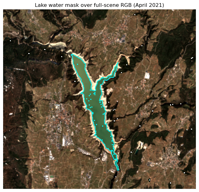

lake_masked = []

for t in range(len(datacube_clear.time)):
    wm = xr.DataArray(
        water_masks[t],
        dims=("y", "x"),
        coords={"y": datacube_clear.y, "x": datacube_clear.x},
        name="water_mask",
    ).rio.write_crs(datacube_clear.rio.crs)

    mask = geometry_mask(
        [lake_gdf.geometry.unary_union],
        transform=wm.rio.transform(),
        invert=True,
        out_shape=wm.shape,
    )
    wm_clipped = wm.where(mask)
    lake_masked.append(wm_clipped)

water_masks_clipped = xr.concat(lake_masked, dim="time")

water_fraction = water_masks_clipped.sum(dim=("y", "x")) / (
    water_masks_clipped.notnull().sum(dim=("y", "x"))
)

Water surface area extraction¶

df_water = pd.DataFrame(
    {"time": water_fraction.time.values, "water_fraction": water_fraction.values}
)
df_water.set_index("time", inplace=True)

pixel_area_m2 = 20 * 20

water_pixel_count = (water_masks_clipped == 1).sum(dim=("y", "x"))
water_area_m2 = water_pixel_count * pixel_area_m2

water_area_m2 = water_area_m2.assign_coords(time=water_masks_clipped.time)

dates = pd.to_datetime(water_masks.time.values)

water_area_ts = pd.Series(water_area_m2.values, index=dates)

smoothed = water_area_ts.rolling(window=5, center=True, min_periods=1).mean()

plt.figure(figsize=(12, 5))
plt.plot(
    water_area_ts.index,
    water_area_ts.values / 1e6,
    color="lightgray",
    alpha=0.6,
    label="Raw",
)
plt.plot(
    smoothed.index,
    smoothed.values / 1e6,
    color="blue",
    linewidth=2,
    label="rolling mean",
)
plt.ylabel("Lake surface area (km²)")
plt.xlabel("Date")
plt.title("Lake surface area over time")
plt.grid(True, linestyle="--", alpha=0.6)
plt.legend()
plt.show()

cluster.shutdown()

Welcome

Random Forest Based Land-Cover Mapping with Sentinel-2

Welcome

Tutorials